LLMs From Scratch Day 9

This is another long-overdue update; a more appropriate title is probably days 9-11, but that's beside the point. Over a few working sessions I debugged/rewrote various parts of the codebase, and finally got to the point where models are training.

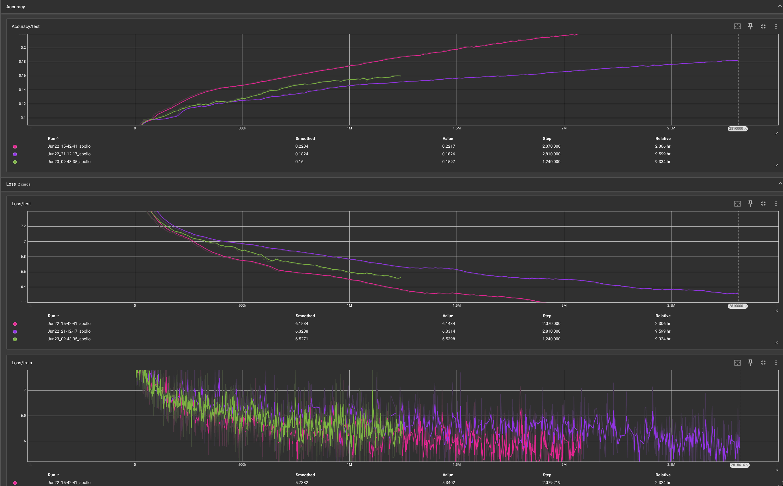
In this post, I'll do my best to cover the major changes that I had to make and the additions since my last post.

First, I got rid of all the activation functions from the dictionary(ies) that were holding model parameters. I initially included them because I wanted to be able to modify the networks by changing the constructor functions rather than modifying the forward pass function, which seemed cleaner. But those functions are static, so we don't want their gradients, and Jax will complain if the functions are already jit'ed. Moving the activation functions to the forward pass eliminated that issue and in retrospect this was clearly the best way to do it from the start using Jax. Another minor issue I fixed was usage of ReLU instead of LayerNorm in between sub-layers. For some reason, I had it in my head that ReLU was used between each sub-layer, as well as in between the feed-forward layers, but it's actually only used with the feed-forward. LayerNorm is used between sublayers, which I realized while rereading Attention Is All You Need to get their hyperparameters.

That leads me to a second change I made: modifying the network hyperparameters and adding a learning rate scheduler. On my first attempt at training, I used the Karpathy method of overfitting a single batch. This worked well for a relatively long time, but eventually the loss exploded to NaN. The issue was a relatively simple fix, namely clipping gradients and dropping the learning rate. After that overfitting the first batch worked as expected, so I made a first attempt at training. I was not using the full 6 layers of encoder/decoder, I was only using 2 and my model still went OOM. I don't have a huge GPU (16GB) so this isn't a unexpected result, but it was a bit disappointing as it means I likely won't be able to train the full model from AIAYN without spending some money on compute. Either way, I dropped a few of the hyperparameters that had a large impact on memory -- $d_{model}$, $heads$, $max\_sequence\_length$ -- and trained on a much smaller footprint.

This worked, and my smalled model was training, at which point I stopped it to add in the learning rate scheduler. The formula is pretty simple, but it relies on $timesteps$, which in turn is impacted by batch size and the max sequence length. The reason for this is, in the paper, the authors state that each batch contained about 25,000 input and output tokens each. The reason for fixing on a token number and not batch size is intuitive: first, memory scales with both batch size and sequence length, so a smaller batch of inputs with longer sequence lengths uses the same memory as a larger batch with shorter sequence lengths. In principal you want to maximize the amount of vRAM utilization throughout your training, but that requires stepping batch sizes up and down accordingly based on the sequence length required of said batch (note: I did not bother using different sequence legnths up to this point, I just pad or trim to the max sequence length. This makes the dataloader code simpler, but it also makes Jax much faster, because you don't need to recompile based on a new sequence length in your input). Second, recall that the model is learning to predict the $N+1$ token with $N$ previous tokens, so within a single input you're predicting $P(t[1] | t[0]), P(t[2] | t[0,1]), ...)$ where $t$ is the token sequence. That means that the total number of input output pairs is really more like $batch\_size * (max\_sequence\_length - 1)$, again highlighting that batch size and sequence length both play a role in the memory consumption of the model.

All that means that each timestep for the base model in the paper correspondeds with about 25,000 samples to learn from, whereas my model only has 8 * 64 = 512 in the small model case! Granted, the small model has many less parameters, so it may not need the full schedule that the full model needs. Either way, I think the easiest way to solve this -- especially as I try and push the model to larger sizes -- is normalize a timestep to denote the passage of 25,000 tokens, not each batch independently. I could also implement gradient accumulation, though I'd like to train before I do that so I can more easily compare its impact to not using it.

So, what's left to do? Well, first things first I need to see how large of a model I can actually get before I run out of memory, and see if that's close to anything test in the paper. Ultimately I'd like to compare my results to theirs to see how close I can get. I still need to normalize the timesteps like I described above, and I need to implement the metrics used in the paper (BLEU), although depending on the difficulty that presents I may just use an existing implementation. Finally, it would be nice to actually do inference with my model! So I'll need to implement a loop that cycles the generated tokens through the decoder until we hit $<eos>$. I could implement KV Caching from scratch to help with that process, but for now I want to focus on training.

See you in day 10 as I tighten up training!